too-many-cells
Table of Contents
- Description
- New interactive release with Python implementation
- New features for v3.0.0.0
- New features for v2.2.0.0
- New features for v2.0.0.0
- New features since initial launch
- Installation
- Troubleshooting
- Using nix, I’m getting shared object not found errors.
- I am getting errors like
AesonException "Error in $.packages.cassava.constraints.flags...when runningstackcommands - I use conda or custom ld library locations and I cannot install
too-many-cellsor run into weird R errors - I am still having issues with installation
- I am on macOS/Windows with docker and
too-many-cellssilently crashes. - I am getting the error
--draw-leafcannot be read, but I copied the command!
- Included projects
- Usage
- Advanced documentation
- Demo
See https://github.com/GregorySchwartz/too-many-cells for latest version. See
too-many-peaks for more information about scATAC-seq usage. See spatial for
more information about spatial usage.
See the publication (and please cite!) for more information about the algorithm.
Description
too-many-cells is a suite of tools, algorithms, and visualizations focusing on
the relationships between cell clades. This includes new ways of clustering,
plotting, choosing differential expression comparisons, and more! While
too-many-cells was intended for single cell RNA-seq, any abundance data in any
domain can be used. Rather than opt for a unique positioning of each cell using
dimensionality reduction approaches like t-SNE, UMAP, and LSA, too-many-cells
recursively divides cells into clusters and relates clusters rather than
individual cells. In fact, by recursively dividing until further dividing would
be considered noise or random partitioning, we can eliminate noisy relationships
at the fine-grain level. The resulting binary tree serves as a basis for a
different perspective of single cells, using our birch-beer visualization
and tree measures to describe simultaneously large and small populations,
without additional parameters or runs. See below for a full list of features.
New interactive release with Python implementation
- A new interactive version of TooManyCells, TooManyCellsInteractive, was launched! Check it out at https://github.com/schwartzlab-methods/too-many-cells-interactive, with the relevant publication at https://academic.oup.com/gigascience/article/doi/10.1093/gigascience/giae056/7738847.
- A new Python implementation of the clustering process, TooManyCells (à la Python), was released at https://github.com/schwartzlab-methods/too-many-cells-python, fully compatible with AnnData objects (and TooManyCellsInteractive)!
New features for v3.0.0.0
- Added new
spatialentry point for spatial analysis of cells! Can make interactive plots of the cells in-situ with their features as well as quantify spatial relationships between pairs of cells. - Overhauled the command line interface, so expect to find possible instability with the options. Open an issue at https://github.com/GregorySchwartz/too-many-cells/issues if you encounter any expected errors or behavior!
- Added MinMaxNorm for min-max normalization and TransposeNorm to transpose the
matrix to apply normalizations back and forth between axes, for instance,
--normalization QuantileNorm --normalization TransposeNorm --normalization
  MinMaxNorm --normalization TransposeNorm
will first apply quantile normalization to each cell, then min-max normalization to each column (before returning the cells to the proper axis with another tranpose). - Incompatibility: Projection file format changed “barcode” column to “item”.
New features for v2.2.0.0
--no-edgerreplaced with--edgeras the default is now Kruskal-Wallis.- Can now use backgrounds for motifs.
- Can specify motif for genome analysis (i.e.
findMotifsGenome.plfrom HOMER). - Temporary directories are now variables to correctly specify location.
- Added q-values for differential.
- Updated documentation for
too-many-peaks.
New features for v2.0.0.0
- Support for scATAC-seq for chromatin state relationships with
too-many-peaks! - Find enchriched regions as peaks for scATAC-seq with
peaks. - Find motifs from differential chromatin state using
motifs. - Linear relationships across the tree as pseudotime with
paths. - Classify single-cell data from bulk with
classify. - New dimensionality reductions with
--lsa. - Output transformed matrix with
matrix-output. - Bypass
labels.csvwith-Zquick labels. - MADs-from-median-based thresholds for multi-gene overlay plots
- Multiple normalization application
- And much more!
New features since initial launch
- Now packaged for the functional package manager
nix(Linux only)! No more dependency shuffling or root for Docker needed! - A new R wrapper was written to quickly get data to and from
too-many-cellsfrom R. Check it out here! - Now works with Cellranger 3.0 matrices in addition to Cellranger 2.0
- Can prune (make into leaves) specified nodes with
--custom-cut. - Can analyze sets of features averaged together (e.g. gene sets). Breaks API,
so update your
--draw-leaf "DrawItem (DrawContinuous \"Cd4\")"argument to--draw-leaf "DrawItem (DrawContinuous [\"Cd4\"])"(notice the list notation). - Outputs values from differential entry point plots (from
--features), and can aggregate features by average.
Installation
We provide multiple ways to install too-many-cells. We recommend installing
with nix . nix will provide all dependencies in the build, supports Linux,
and should be reproducible, so try that first. We also have docker images and a
Dockerfile to use in any system in case you have a custom build (for instance,
a non-standard R installation) or difficulty installing. macOS and Windows
users: too-many-cells was built and tested on Linux, so we highly recommend
using the docker image (which is a completely isolated environment which
requires no compiling or installation, other than docker itself) as there may be
difficulties in installing the dependencies.
nix
too-many-cells can be installed using the functional package manager nix .
While you will need sudo to install, no sudo is required after the correct
setup. First, install nix following the instructions
on the website. Then, with an unset LD_LIBRARY_PATH,
git clone https://github.com/GregorySchwartz/too-many-cells.git
cd too-many-cells
nix-env -f default.nix -i too-many-cells
Stack (unsupported in too-many-cells >= v2.0.0.0, use nix)
Dependencies
You may require the following dependencies to build and run (from Ubuntu 14.04, use the appropriate packages from your distribution of choice):
- build-essential
- libgmp-dev
- libblas-dev
- liblapack-dev
- libgsl-dev
- libgtk2.0-dev
- libcairo2-dev
- libpango1.0-dev
- graphviz
- r-base
- r-base-dev
To install them, in Ubuntu:
sudo apt install build-essential libgmp-dev libblas-dev liblapack-dev libgsl-dev libgtk2.0-dev libcairo2-dev libpango1.0-dev graphviz r-base r-base-dev
too-many-cells also uses the following packages from R:
- cowplot
- ggplot2
- edgeR
- jsonlite
To install them in R,
install.packages(c("ggplot2", "cowplot", "jsonlite"))
install.packages("BiocManager")
BiocManager::install("edgeR")
Install stack
See https://docs.haskellstack.org/en/stable/README/ for more details.
curl -sSL https://get.haskellstack.org/ | sh
stack setup
Install too-many-cells
- Source
Probably the easiest method if you don’t want to mess with dependencies (outside of the ones above).
git clone https://github.com/GregorySchwartz/too-many-cells.git cd too-many-cells stack install - Online
We only require
stack(orcabal), you do not need to download any source code (but you might need the stack.yaml.old dependency versions), just run the following command to placetoo-many-cells < v2.0.0.0in your~/.local/bin/:mv stack.yaml.preV2 stack.yaml stack install too-many-cells
If you run into errors like
Error: While constructing the build plan, the
following exceptions were encountered:
, then follow the advice. Usually you just need to follow the suggestion and add the dependencies to the specified file. For a quickyamlconfiguration, refer to https://github.com/GregorySchwartz/too-many-cells/blob/master/stack.yaml.old. - macOS
We recommend using docker on macOS. The following is written for
too-many-cells < v2.0.0.0. If you must compiletoo-many-cells, you should get the above dependencies. For some dependencies, you can use brewer, then installtoo-many-cells(in the cloned folder, don’t forget to install the R dependencies above):brew cask install xquartz brew install glib cairo gtk gettext fontconfig freetype brew tap brewsci/bio brew tap brewsci/science brew install r zeromq graphviz pkg-config gsl libffi gobject-introspection gtk+ gtk+3 # Needed so pkg-config and libraries can be found. # For the second path, use the ouput of "brew info libffi". export PKG_CONFIG_PATH=/usr/local/lib/pkgconfig:/usr/local/opt/libffi/lib/pkgconfig # Tell gtk that it's quartz stack install --flag gtk:have-quartz-gtk
Docker
Different computers have different setups, operating systems, and repositories.
Do put the entire program in a container to bypass difficulties (with the other
methods above), we user docker. So first, install docker.
To get too-many-cells (replace 2.0.0.0 with any version needed):
docker pull gregoryschwartz/too-many-cells:2.0.0.0
To run too-many-cells in a docker container:
sudo docker run -it --rm -v "/home/username:/home/username" gregoryschwartz/too-many-cells:2.0.0.0 -h
Now you can follow the tutorial below with the addition of the docker paths and
commands. If you add yourself to the docker group, sudo is not needed. For instance:
docker run -it --rm -v "/home/username:/home/username" \
    gregoryschwartz/too-many-cells:2.0.0.0 make-tree \
    --matrix-path /home/username/path/to/input \
    --labels-file /home/username/path/to/labels.csv \
    --draw-collection "PieRing" \
    --output /home/username/path/to/out \
    > clusters.csv
Make sure to increase the memory that can be used by docker containers if you
use macOS or Windows. Also, docker won’t be able to find your files by default.
You need to mount the folders with -v in order to have docker read and write
from and to the filesystem, respectively. Read the documentation about volumes
for more information. You can simply mount your entire relevant path as in the
above example to handle both input and output, or just mount your entire user
directory as above. Specifically, -v "/home/username:/home/username" for the
whole directory or each individual -v /path/to/matrix/on/host:/input_matrix
with -m /input_matrix is what you want, where before the : is on the host
filesystem while after the : is what the docker program sees. Then you can
write the output in the same way: -v /path/to/output/on/host:/output will
write the output to the folder before the :.
To build the too-many-cells image yourself if you want:
nix-build docker.nix
docker load < /nix/store/${NAME_OF_OUTPUT_IMAGE}.tar.gz
Troubleshooting
Using nix, I’m getting shared object not found errors.
Be sure to have LD_LIBRARY_PATH unset when running nix-env to make sure the
linked libraries are in /nix/store.
I am getting errors like AesonException "Error in $.packages.cassava.constraints.flags... when running stack commands
Try upgrading stack with stack upgrade. The new installation will be in
~/.local/bin, so use that binary.
I use conda or custom ld library locations and I cannot install too-many-cells or run into weird R errors
stack and too-many-cells assume system libraries and programs. To solve this
issue, first install the dependencies above at the system level, including
system R. Then to every stack and too-many-cells command, prepend
PATH="$HOME/.local/bin:/usr/bin:$PATH" to all commands. For instance:
PATH="$HOME/.local/bin:/usr/bin:$PATH" stack installPATH="$HOME/.local/bin:/usr/bin:$PATH" too-many-cells make-tree -h
If your shared libraries are abnormal and use libR.so from non-system
locations, be sure to also have LD_LIBRARY_PATH=/usr/lib/:$LD_LIBRARY_PATH
when installing (and / or the location of R libraries, such as
/usr/local/lib/R/lib/).
I am still having issues with installation
Open an issue! While working on the issue, try out the docker for
too-many-cells, it requires no installation at all (other than docker).
I am on macOS/Windows with docker and too-many-cells silently crashes.
Docker containers may run into this issue if the memory given to the containers is insufficient. Make sure to increase the memory that can be used by docker containers.
I am getting the error --draw-leaf cannot be read, but I copied the command!
For some computers, you may need to change the command to single quotations for
the argument: --draw-leaf 'DrawItem (DrawContinuous [\"Cd4\"])'
Included projects
This project is a collection of libraries and programs written specifically for
too-many-cells:
-
birch-beer - Generate a tree for displaying a hierarchy of groups with colors, scaling, and more.
-
modularity - Find the modularity of a network.
-
spectral-clustering - Library for spectral clustering.
-
hierarchical-spectral-clustering - Hierarchical spectral clustering of a graph.
-
differential - Finds out whether an entity comes from different distributions (statuses).
Usage
too-many-cells has several entry points depending on the desired analysis.
| Argument | Analysis |
|---|---|
make-tree |
Generate the tree from single cell data with various measurement outputs and visualize tree |
interactive |
Interactive visuzalization of the tree, very slow |
differential |
Find differentially expressed features between two nodes |
diversity |
Conduct diversity analyses of multiple cell populations |
paths |
The binary tree equivalent of the so called “pseudotime”, or 1D dimensionality reduction |
The main workflow is to first generate and plot the population tree using
too-many-cells make-tree, then use the rest of the entry points as needed.
At any point, use -h to see the help of each entry point.
Also, check out tooManyCellsR for an R wrapper!
make-tree
too-many-cells make-tree generates a binary tree using hierarchical spectral
clustering. We start with all cells in a single node. Spectral clustering
partitions the cells into two groups. We assess the clustering using
Newman-Girvan modularity: if \(Q > 0\) then we recursively continue with
hierarchical spectral clustering. If not, then there is only a single community
and we do not partition – the resulting node is a leaf and is considered the
finest-grain cluster.
The most important argument is the –prior argument. Making the tree may
take some time, so if the tree was already generated and other analysis or
visualizations need to be run on the tree, point the --prior argument to the
output folder from a previous run of too-many-cells. If you do not use
--prior, the entire tree will be recalculated even if you just wanted to
change the visualization!
The main input is the --matrix-path argument. When a directory is supplied,
too-many-cells interprets the folder to have matrix.mtx, genes.tsv, and
barcodes.tsv files (cellranger outputs, see cellranger for specifics). If
a file is supplied instead of a directory, we assume a csv file containing
feature row names and cell column names. This argument can be called multiple times
to combine multiple single cell matrices: --matrix-path input1 --matrix-path
input2.
The second most important argument is --labels-file. Supply with a csv with
a format and header of “item,label” to provide colorings and statistics of the
relationships between labels. Here the “item” column contains the name of each
cell (barcode) and the label is any property of the cell (the tissue of origin,
hour in a time course, celltype, etc.). You can also now use -Z as a list for
each matching -m in order to manually give the entire matrix that label
(useful for situations like -m ./t-all -Z T-ALL -m ./control -Z Control). To
get the newly generated labels with =-Z into a labels.csv file, specify
--labels-output and the labels.csv will be in the output folder.
To see the full list of options, use too-many-cells -h and -h for each entry
point (i.e. too-many-cells make-tree -h).
Output
too-many-cells make-tree generates several files in the output folder. Below
is a short description of each file.
| File | Description |
|---|---|
clumpiness.csv |
When labels are provided, uses the clumpiness measure to determine the level of aggregation between each label within the tree. |
clumpiness.pdf |
When labels are provided, a figure of the clumpiness between labels. |
cluster_diversity.csv |
When labels are provided, the diversity, or “effective number of labels”, of each cluster. |
cluster_info.csv |
Various bits of information for each cluster and the path leading up to each cluster, from that cluster to the root. For instance, the size column has cluster_size/parent_size/parent_parent_size/.../root_size |
cluster_list.json |
The json file containing a list of clusterings. |
cluster_tree.json |
The json file containing the output tree in a recursive format. |
dendrogram.svg |
The visualization of the tree. There are many possible options for this visualization included. Can rename to choose between PNG, PS, PDF, and SVG using --dendrogram-output. |
graph.dot |
A dot file of the tree, with less information than the tree in cluster_results.json. |
node_info.csv |
Various information of each node in the tree. |
projection.pdf |
When --projection is supplied with a file of the format “barcode,x,y”, provides a plot of each cell at the specified x and y coordinates (for instance, when looking at t-SNE plots with the same labelings as the dendrogram here). |
Outline with options
The basic outline of the default matrix pre-processing pipeline with some
relevant options is as follows (there are many additional options including cell
whitelists that can be seen using too-many-cells make-tree -h):
- Read matrix.
- Optionally remove cells with less than X counts (
--filter-thresholds). - Optionally remove features with less than X count (
--filter-thresholds). - Term frequency-inverse document frequency normalization (
--normalization). - Optionally use dimensionality reduction (
--lsa). - Finish.
Example
- Setup
We start with our input matrix. Here,
ls ./input
barcodes.tsv genes.tsv matrix.mtx
Note that the input can be a directory (with the
cellrangermatrix format above) or a file (acsvfile). You can also point to acellranger>= 3.0 folder which hasmatrix.mtx.gz,features.tsv.gz, andbarcodes.tsv.gzfiles instead. You don’t need to use scRNA-seq data! You can use any data that has observations (cells) and features (genes), as long as you agree that the observations are related by their feature abundances. If you do upstream batch effect correction, LSA, normalization, or anything else, be sure to use--normalization NoneNorm(and--shift-positivefor LSA) to avoid wrong filters and scalings! If using dimensionality reduction such as PCA and t-SNE, we highly recommend generating your own similarity matrix for use with ourcluster-treeprogram and plot withbirch-beer, as we emphasize a feature matrix intoo-many-cellsand dimensionality reduction algorithms transform counts (our input which works with cosine similarity) into more nebulous information (which may not work with cosine similarity).cluster-tree, however, can be used with adjacency and similarity matrices. As for formats, the matrix market format contains three files like so:The
matrix.mtxfile is in matrix market format.%%MatrixMarket matrix coordinate integer general % 23433 1981 4255069 4 1 1 5 1 1 11 1 2 23 1 2 25 1 2 40 1 2 48 1 1 ...
The
genes.tsvfile (orfeatures.tsv.gz) contains the features of each cell and corresponds to the rows ofmatrix.mtx. Here, both columns were the same gene symbols, but you can have Ensembl as the first column and gene symbol as the second, etc. The columns and column orders don’t matter, but make sure all matrices have the same format and specify the symbols you want to use (for overlaying gene expression, differential expression, etc.) with--feature-column COLUMN. So to use the second column for gene expression, you would use--feature-column 2.Xkr4 Xkr4 Rp1 Rp1 Sox17 Sox17 Mrpl15 Mrpl15 Lypla1 Lypla1 Tcea1 Tcea1 Rgs20 Rgs20 Atp6v1h Atp6v1h Oprk1 Oprk1 Npbwr1 Npbwr1 ...
The
barcodes.tsvfile contains the ids of each cell or observation and corresponds to the columns ofmatrix.mtx.AAACCTGCAGTAACGG-1 AAACGGGAGAAGAAGC-1 AAACGGGAGACCGGAT-1 AAACGGGAGCGCTCCA-1 AAACGGGAGGACGAAA-1 AAACGGGAGGTACTCT-1 AAACGGGAGGTGCTTT-1 AAACGGGAGTCGAGTG-1 AAACGGGCATGGTCAT-1 AAAGATGAGCTTCGCG-1 ...
For a
csvfile, the format is dense (observation columns (cells), feature rows (genes)):"","A22.D042044.3_9_M.1.1","C5.D042044.3_9_M.1.1","D10.D042044.3_9_M.1.1","E13.D042044.3_9_M.1.1","F19.D042044.3_9_M.1.1","H2.D042044.3_9_M.1.1","I9.D042044.3_9_M.1.1",... "0610005C13Rik",0,0,0,0,0,0,0,... "0610007C21Rik",0,112,185,54,0,96,42,... "0610007L01Rik",0,0,0,0,0,153,170,... "0610007N19Rik",0,0,0,0,0,0,0,... "0610007P08Rik",0,0,0,0,0,19,0,... "0610007P14Rik",0,58,0,0,255,60,0,... "0610007P22Rik",0,0,0,0,0,65,0,... "0610008F07Rik",0,0,0,0,0,0,0,... "0610009B14Rik",0,0,0,0,0,0,0,... ...
We also know where each cell came from, so we mark that down as well in a
labels.csvfile.item,label AAACCTGCAGTAACGG-1,Marrow AAACGGGAGACCGGAT-1,Marrow AAACGGGAGCGCTCCA-1,Marrow AAACGGGAGGACGAAA-1,Marrow AAACGGGAGGTACTCT-1,Marrow ...
This can be easily accomplished with
sed:cat barcodes.tsv | sed "s/-1/-1,Marrow/" | s/-2/etc... > labels.csvFor
cellranger, note that the-1,-2, etc. postfixes denote the first, second, etc. label in the aggregationcsvfile used as input forcellranger aggr. - Default run
We can now run the
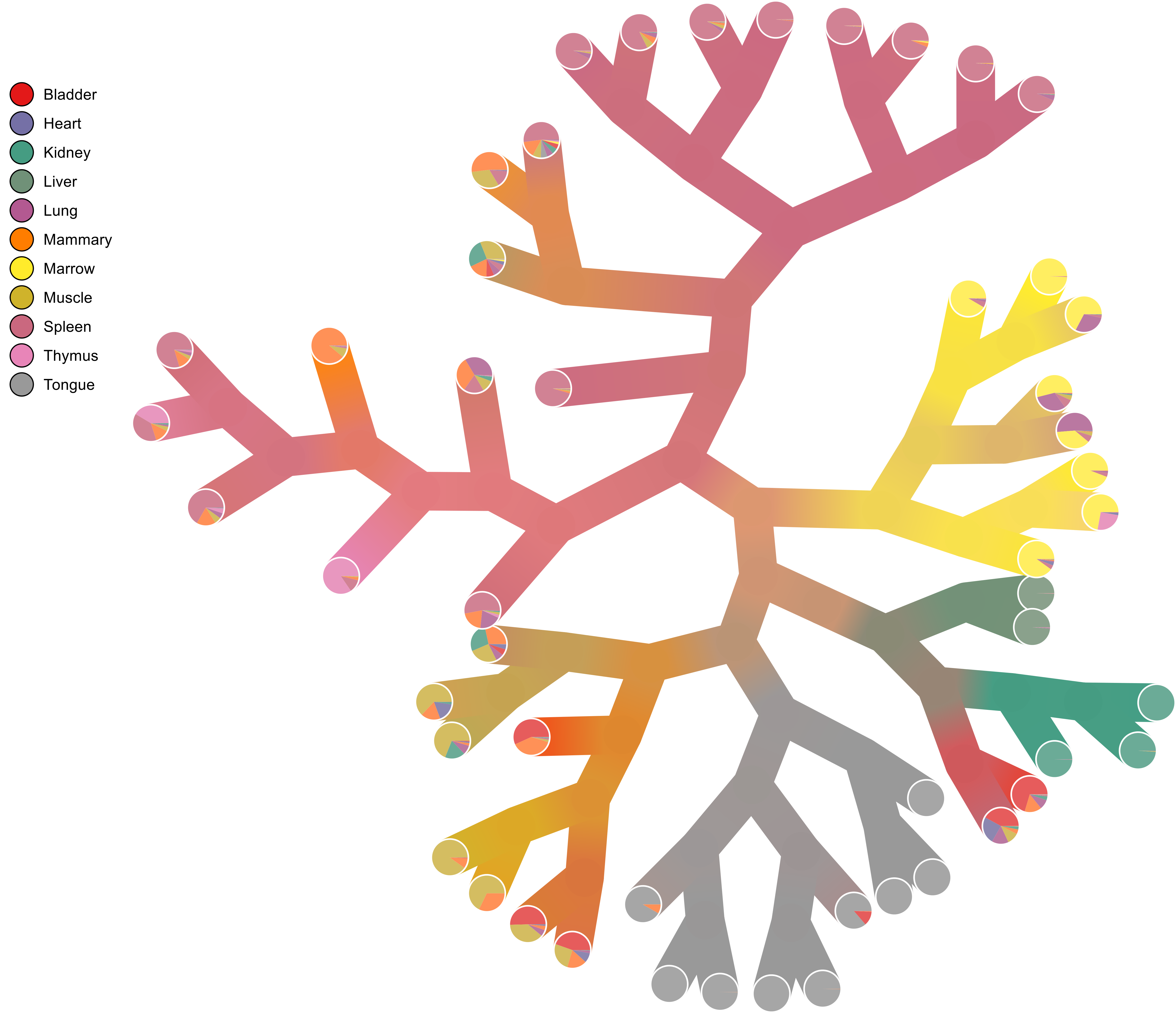
too-many-cellsalgorithm on our data. The resulting cells with assigned clusters will be printed tostdout(don’t forget to use--normalization NoneNormon preprocessed data, as stated here). While older versions had default filter thresholds for (MINCELL, MINFEATURE) counts, sincev2.0.0.0the default is now no filtering to account for multiple assay types.too-many-cells make-tree \ --matrix-path input \ --labels-file labels.csv \ --filter-thresholds "(250, 1)" \ --draw-collection "PieRing" \ --output out \ > clusters.csv
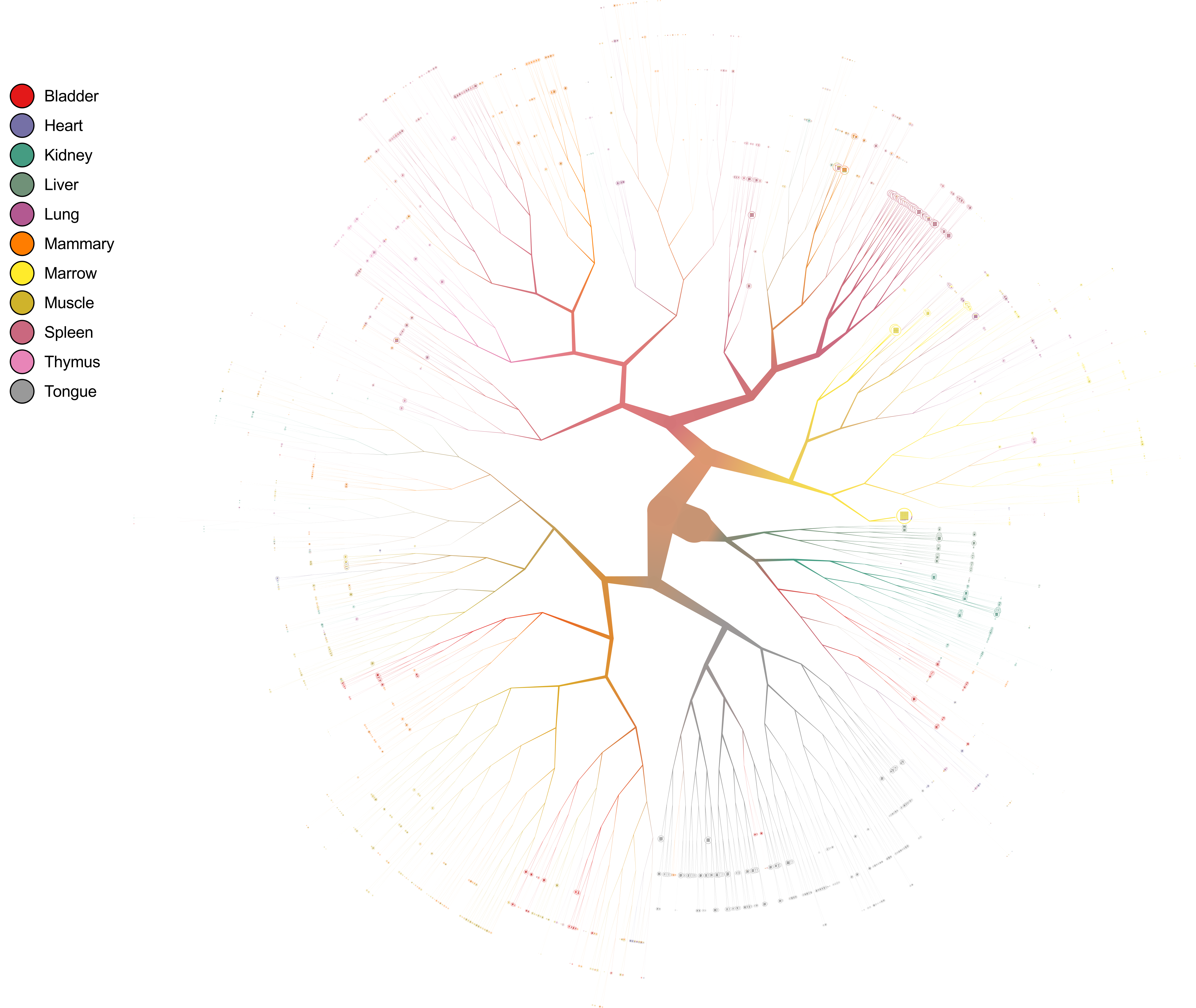
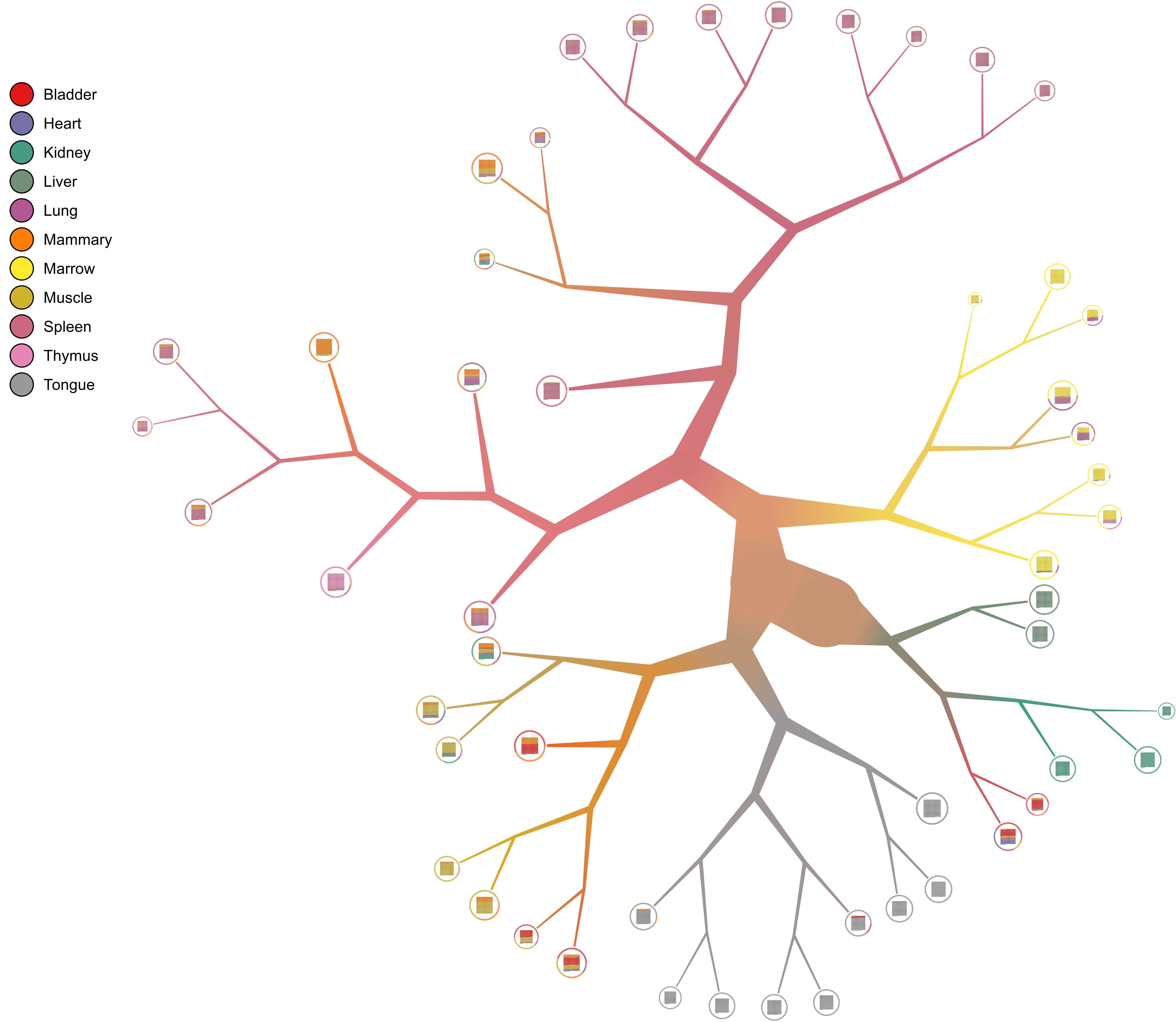
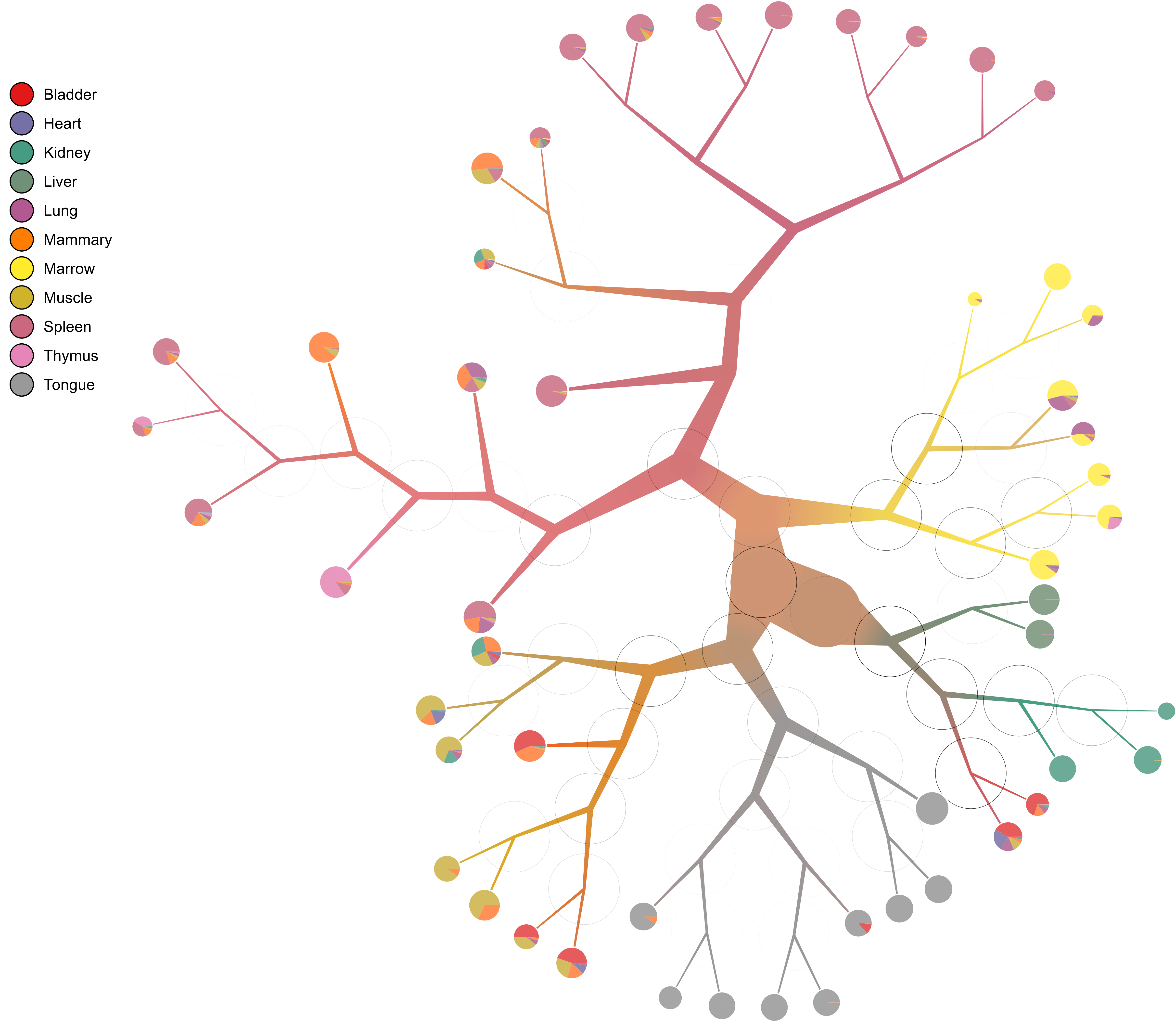
- Pruning tree
Large cell populations can result in a very large tree. What if we only want to see larger subpopulations rather than the large (inner nodes) and small (leaves)? We can use the
--min-size 100argument to set the minimum size of a leaf to 100 in this case. Alternatively, we can specify--smart-cutoff 4in addition to--min-size 1to set the minimum size of a node to \(4 * \text{median absolute deviation (MAD)}\) of the nodes in the original tree. Varying the number of MADs varies the number of leaves in the tree.--smart-cutoffshould be used in addition to--min-size,--max-proportion,--min-distance, or--min-distance-searchto decide which cutoff variable to use. The value supplied to the cutoff variable is ignored when--smart-cutoffis specified. We’ll prune the tree for better visibility in this document.Note: the pruning arguments change the tree file, not just the plot, so be sure to output into a different directory.
Also, we do not need to recalculate the entire tree! We can just supply the previous results using
--prior(we can also remove--matrix-pathwith--priorto speed things up, but miss out on some features if needed):too-many-cells make-tree \ --prior out \ --labels-file labels.csv \ --smart-cutoff 4 \ --min-size 1 \ --draw-collection "PieRing" \ --output out_pruned \ > clusters_pruned.csv
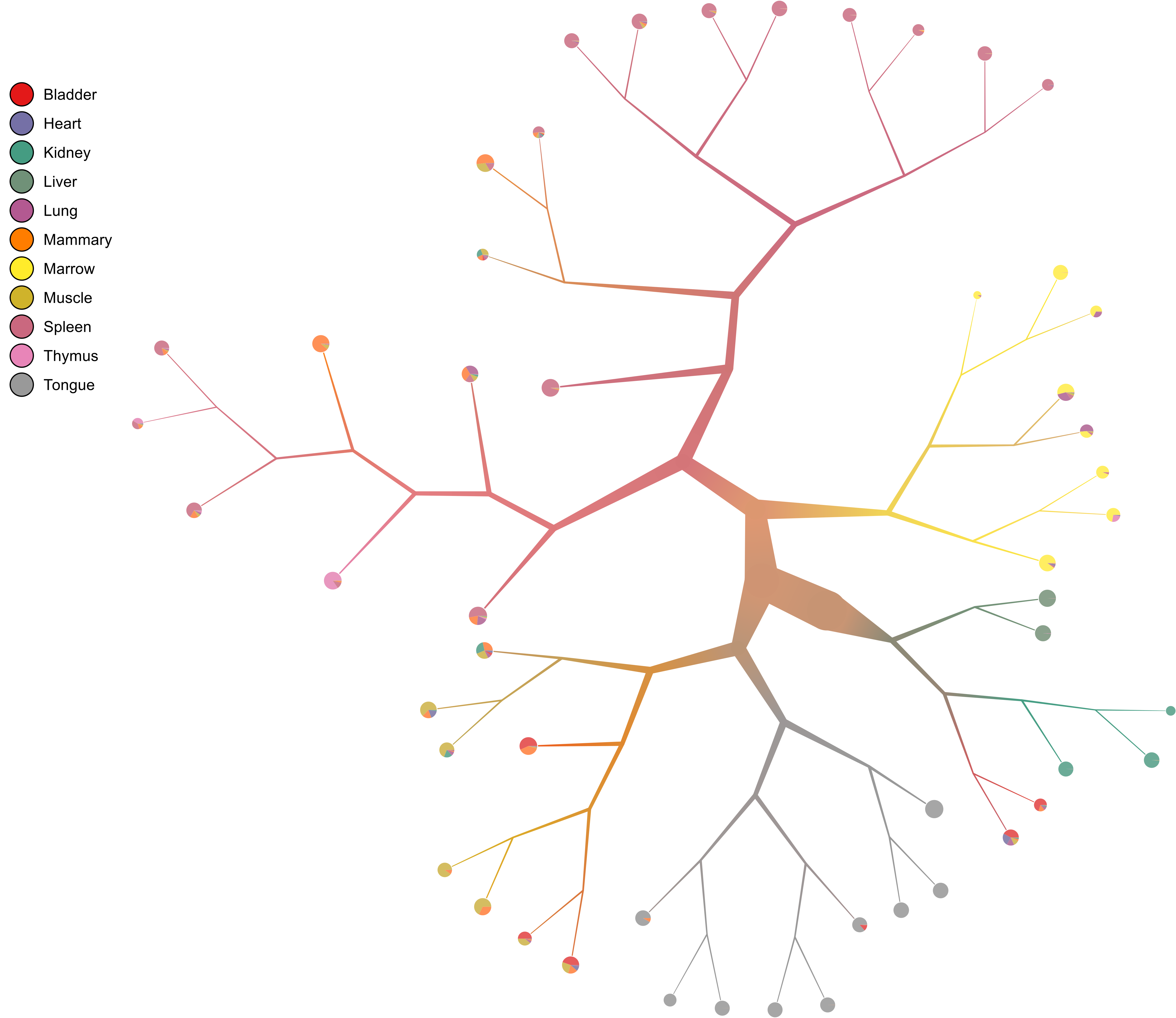
- Pie charts
What if we want pie charts instead of showing each individual cell (the default)?
too-many-cells make-tree \
    --prior out \
    --labels-file labels.csv \
    --smart-cutoff 4 \
    --min-size 1 \
    --draw-collection "PieChart" \
    --output out_pruned \
    > clusters_pruned.csv

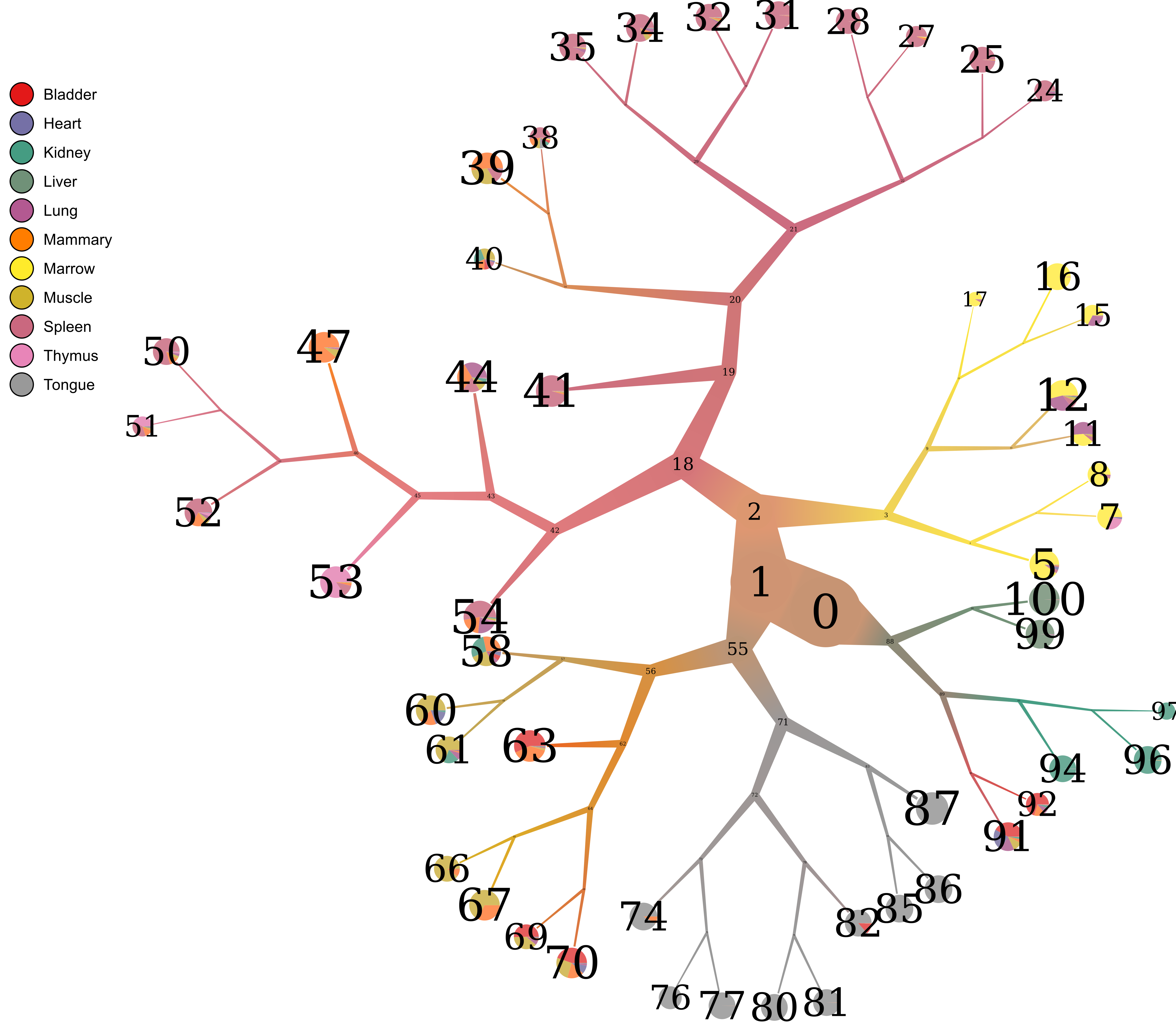
- Node numbering
Now that we see the relationships between clusters and nodes in the dendrogram, how can we go back to the data – which nodes represent which node IDs in the data?
too-many-cells make-tree \
    --prior out \
    --labels-file labels.csv \
    --smart-cutoff 4 \
    --min-size 1 \
    --draw-collection "PieChart" \
    --draw-node-number \
    --output out_pruned \
    > clusters_pruned.csv
- Branch width
We can also change the width of the nodes and branches, for instance if we want thinner branches:
too-many-cells make-tree \
    --prior out \
    --labels-file labels.csv \
    --smart-cutoff 4 \
    --min-size 1 \
    --draw-collection "PieChart" \
    --draw-max-node-size 40 \
    --output out_pruned \
    > clusters_pruned.csv
- No scaling
We can remove all scaling for a normal tree and still control the branch widths:
too-many-cells make-tree \
    --prior out \
    --labels-file labels.csv \
    --smart-cutoff 4 \
    --min-size 1 \
    --draw-collection "PieChart" \
    --draw-max-node-size 40 \
    --draw-no-scale-nodes \
    --output out_pruned \
    > clusters_pruned.csv
How strong is each split? We can tell by drawing the modularity of the children on top of each node:
too-many-cells make-tree \
    --prior out \
    --labels-file labels.csv \
    --smart-cutoff 4 \
    --min-size 1 \
    --draw-collection "PieChart" \
    --draw-mark "MarkModularity" \
    --output out_pruned \
    > clusters_pruned.csv
- Gene expression
What if we want to draw the gene expression onto the tree in another folder (requires
--matrix-path, may take some time depending on matrix size. Defaults to all black if the feature name is not present in the matrix, so check the first column of the feature file)? Note: the feature names are from thegenes.tsvorfeatures.tsv.gzfile. Usually,cellrangerhas Ensembl identifiers as the first column and gene symbol as the second column, so if you want to specify gene symbol, use--feature-column 2(1 is default).too-many-cells make-tree \ --prior out \ --matrix-path input \ --labels-file labels.csv \ --filter-thresholds "(250, 1)" \ --smart-cutoff 4 \ --min-size 1 \ --feature-column 2 \ --draw-leaf "DrawItem (DrawContinuous [\"Cd4\"])" \ --output out_gene_expression \ > clusters_pruned.csv
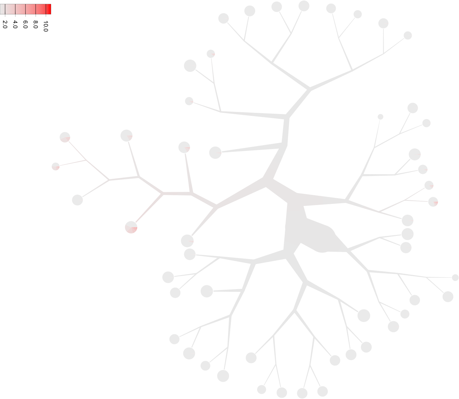
Notice that Cd4 is within a list ([]), so multiple features can be listed and the average of those values for each cell will be used. While this representation shows the expression of Cd4 in each cell and blends those levels together, due to the sparsity of single cell data these cells and their respective subtrees may be hard to see without additional processing. Let’s scale the saturation to more clearly see sections of the tree with our desired expression (when choosing other high and low colors with
--draw-colors, scaling the saturation will only affect non-grayscale colors).too-many-cells make-tree \ --prior out \ --matrix-path input \ --labels-file labels.csv \ --filter-thresholds "(250, 1)" \ --smart-cutoff 4 \ --min-size 1 \ --feature-column 2 \ --draw-leaf "DrawItem (DrawContinuous [\"Cd4\"])" \ --draw-scale-saturation 10 --output out_gene_expression \ > clusters_pruned.csv
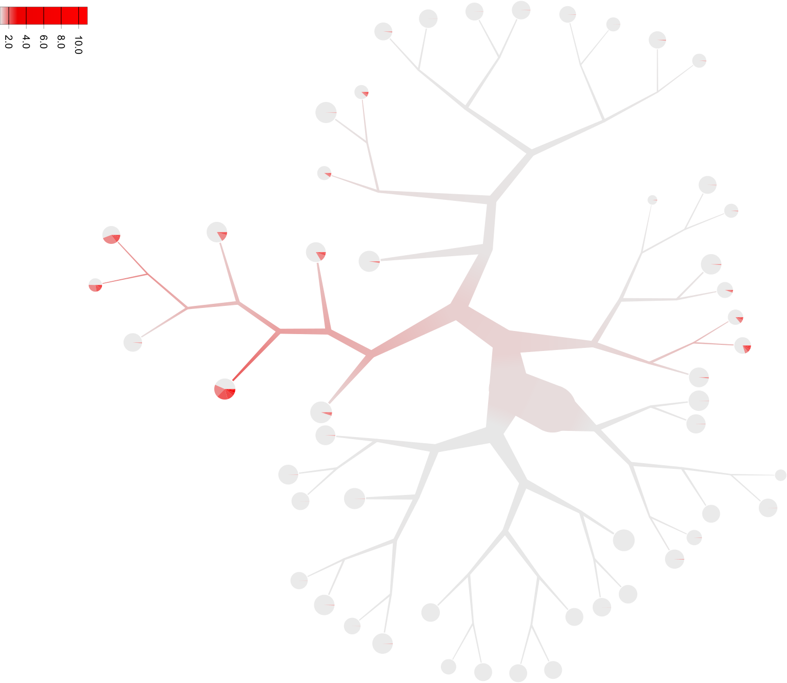
There, much better! Now it’s clearly enriched in the subtree containing the thymus, where we would expect many T cells to be. While this tree makes the expression a bit more visible, there is another tactic we can use. Instead of the continuous color spectrum of expression values, we can have a binary “high” and “low” expression. Here, we’ll continue to have the red and gray colors represent high and low expressions respectively using the
--draw-colorsargument. Note that this binary expression technique can be used for multiple features, hence it’s a list of features with cutoffs (Exactfor specified cutoffs orMadMedianfor how many MADs from the median) so you can be high in a gene and low in another gene, etc. for all possible combinations.too-many-cells make-tree \ --prior out \ --matrix-path input \ --labels-file labels.csv \ --filter-thresholds "(250, 1)" \ --smart-cutoff 4 \ --min-size 1 \ --feature-column 2 \ --draw-leaf "DrawItem (DrawThresholdContinuous [(\"Cd4\", Exact 0), (\"Cd8a\", Exact 0)])" \ --draw-colors "[\"#e41a1c\", \"#377eb8\", \"#4daf4a\", \"#eaeaea\"]" \ --draw-scale-saturation 10 \ --output out_gene_expression \ > clusters_pruned.csv
Now we can see the expression of both Cd4 and Cd8a at the same time!
- Diversity
We can also see an overview of the diversity of cell labels within each subtree and leaves.
too-many-cells make-tree \
    --prior out \
    --matrix-path input \
    --filter-thresholds "(250, 1)" \
    --labels-file labels.csv \
    --smart-cutoff 4 \
    --min-size 1 \
    --draw-leaf "DrawItem DrawDiversity" \
    --output out_diversity \
    > clusters_pruned.csv
Here, the deeper the red, the more diverse (a larger “effective number of cell states”) the cell labels in that group are. Note that the inner nodes are colored relative to themselves, while the leaves are colored relative to all leaves, so there are two different scales.
interactive
The interactive entry point has a basic GUI interface for quick plotting with
a few features. We recommend limited use of this feature, however,
as it can be quite slow at this stage, has fewer customizations, and requires
specific dependencies.
too-many-cells interactive \
    --prior out \
    --labels-file labels.csv
differential
A main use of single cell clustering is to find differential genes between
multiple groups of cells. The differential aids in this endeavor by allowing
comparisons with edgeR. Let’s find the differential genes between the liver
group and all other cells. Consider our pruned tree from earlier:
We can see the id of each group with --draw-node-number.
We need to define two groups to compare. Well, it looks like node 98 defines the
liver cluster. Then, since we don’t want 98 to be in the other group, we say
that all other cells are within nodes 89 and 1. As a result, we end up with a
tuple containing two lists: ([89, 1], [98]). Then our differential genes for
(liver / others) can be found with differential (sent to stdout):
too-many-cells differential \
    --matrix-path input \
    --prior out_pruned \
    --filter-thresholds "(250, 1)" \
    -n "([89, 1], [98])" \
    > differential.csv
If we wanted to make the same comparison, but compare the liver subtree with
liver cells from all other subtrees, we can use the --labels argument:
too-many-cells differential \
    --matrix-path input \
    --prior out_pruned \
    --labels-file labels.csv \
    --filter-thresholds "(250, 1)" \
    -n "([89, 1], [98])" \
    --labels "([\"Liver\"], [\"Liver\"])" \
    > differential_liver.csv
We can also look at the distribution of abundance for individual genes using the
--features and --plot-output arguments.
Furthermore, we can compare each node to all other cells by specifying no nodes
at all. The output file will contain the top --top-n genes for each node. We
recommend using multiple OS threads here to speed up the process using +RTS
-N${NUMOSTHREADS} (no number to use all cores). The following example will
compare all nodes to all other cells using 8 OS threads:
too-many-cells differential \
    --matrix-path input \
    --prior out_pruned \
    --filter-thresholds "(250, 1)" \
    -n "([], [])" \
    --normalization "UQNorm" \
    +RTS -N8
diversity
Diversity is the measure of the “effective number of entities within a system”,
originating from ecology (See Jost: Entropy and Diversity). Here, each cell is
an organism and each cell label or cluster is a species, depending on the
question. In ecology, the diversity index measures the effective number of
species within a population such that the minimum is a diversity of 1 for a
single dominant species up to maximum of the total number of species (evenly
abundant). If our species is a cluster, then here the diversity is the effective
number of cell states within a population (for labels, make-tree generates
these results automatically in “diversity” columns). Say we have two populations
and we generated the trees using make-tree into two different output folders,
out1 and out2. We can find the diversity of each population using the
diversity entry point.
too-many-cells diversity\
    --priors out1 \
    --priors out2 \
    -o out_diversity_stats
We can then find a simple plot of diversity in diversity_output. In addition,
we also provide rarefaction curves for comparing the number of different cell
states at each subsampling useful for comparing the number of cell states where
the population sizes differ.
paths
“Pseudotime” refers to the one dimensional relationship between cells, useful
for looking at the ordering of cell states or labels. The implementation of
pseudotime in a too-many-cells point-of-view is by finding the distance
between all cells and the cells found in the longest path from the root in the
tree. Then each cell has a distance from the “start” and thus we plot those
distances.
too-many-cells paths\
    --prior out \
    --labels-file labels.csv \
    --bandwidth 3 \
    -o out_paths
Working with scATAC-seq data using too-many-peaks
For more information, check out the too-many-peaks walkthrough.
scATAC-seq is a powerful technology for quantifying chromatin accessibility for
individual cells. too-many-cells now supports scATAC-seq to generate cell clade
relationships from chromatin state information through too-many-peaks. All of
the previous analyses used with gene-product features now work with genomic
regions in the form chrN:START-END, where N is the chromosome number,
START is the start of the region and END is the end base of the region.
Matrices in this format can be read from either CSV or matrix-market as
above but with the correctly formatted features, or you can load in directly
from a fragments.tsv.gz file in Cellranger format (tab delimited with each row
being chrN\tSTART\tEND\tBARCODE\tCOUNT) making sure that the filename contains
the fragments ending, such as t-all_fragments.tsv.gz. For example:
too-many-cells make-tree\
    -m ./t-all_fragments.tsv.gz \
    -Z "T-ALL" \
    -m ./control_fragments.tsv.gz
    -Z "Control" \
    --filter-thresholds "(1000, 1)" \
    --binwidth 5000 \
    --lsa 50 \
    --normalization NoneNorm \
    --blacklist-regions-file Anshul_Hg19UltraHighSignalArtifactRegions.bed.gz \
    --draw-node-number \
    --draw-mark "MarkModularity" \
    --fragments-output \
    --labels-output \
    -o out \
    > out_leaves.csv
Note: We use --lsa and --normalization NoneNorm for latent semantic
analysis dimensionality reduction as there are many features in scATAC-seq, so
we try to overcome a potential issue where all cells are considered outliers. To
blacklist known biased regions in the genome, we can call
--blacklist-regions-file. The --fragments-output and --labels-output go
hand-in-hand with -Z in order to keep the renamed barcodes and labels (found
in the output folder). too-many-cells will binarize the data by default unless
--no-binarize is specified. Lastly, we choose a binwidth using --binwidth
to conform to a set of standard features across cells and samples.
peaks
With scATAC-seq, we want to identify enriched locations in the genome for each
newly found subpopulation of cells. The peaks entrypoint can collect the
appropriate fragments for quantification and visualization of peaks.
too-many-cells peaks \
    -f ./out/fragments.tsv.gz \
    --prior ./out \
    --genome human.hg19.genome \
    --bedgraph \
    --labels-file ./out/labels.csv \
    --all-nodes \
    --peak-node "1" \
    --peak-node "5" \
    --peak-node-labels "(1, [\"Control\"])" \
    --peak-node-labels "(5, [\"T-ALL\"])" \
    -o out_peaks \
    +RTS -N6
Here, we will have our peaks in the specified output folder, along with many other files and folder:
| File | Description |
|---|---|
out_peaks/cluster_fragments |
fragments.tsv.gz files for each node. |
out_peaks/cluster_bedgraphs |
Bedgraphs and bigwigs if specified using --bedgraph for track visualization uses. |
out_peaks/cluster_peaks/union.bdg |
Merged peaks across all requested nodes in bedgraph format. |
out_peaks/cluster_peaks/union_fragments.tsv.gz |
Merged peaks across all requested nodes in fragments.tsv.gz format. |
out_peaks/cluster_peaks/ |
Folder containing merged peaks across nodes and peaks for each individual node in each folder. |
--bedgraph enabled the cluster_bedgraphs folder, while --all-nodes
specified to find peaks for all nodes, not just the leaves. However, when paired
with --peak-node, we just look at the peaks for each node in the list (but
--all-nodes is still required if looking at non-leaf nodes as well). Without
--peak-node, this command would have found peaks for every node. Furthermore,
--peak-node-labels allows the filtration based on the label of cells in of the
requested node. --genome tells the peak finding program where the genome file
is (containing the effective genome sizes of chromosomes in tab-delimited format
of chrN\tSIZE used in the MACS2 program). Here, the -f fragments.tsv.gz
and labels.csv was from the previous scATAC-seq section, where we
automatically generated the correctly renamed barcodes and labels. Lastly, +RTS
-N6 tells too-many-cells to use six cores for the calculation. These output
files, especially the merged peak files, can be used for differential
accessibility analysis as in scRNA-seq. This entrypoint is highly customizable,
down to the exact command used for peak calling, so check out too-many-cells
peaks -h for more information.
motifs
After differential accessibility using peaks, the result can be used to find motifs enriched in each node.
too-many-cells motifs \
    --diff-file ./diff_out.csv \
    --motif-genome hg19.fa \
    --top-n 1000 \
    --motif-command "homer/homer-4.9/bin/findMotifs.pl %s fasta %s" \
    -o motifs
In this example, we use the output from a differential expression analysis using
too-many-cells differential from our merged peaks. Using a complete genome
file used by our motif program of choice (here HOMER, but defaults to MEME) with
--motif-genome, we want to provide the motif program with the top 1000 most
differential peaks using --top-n. Lastly, while the default uses MEME, we find
HOMER to be much faster. The prior command shows the use of another program to
find the motifs, making sure the %s for input and output are in the right
locations (check too-many-cells motifs -h).
classify
To identify potential cell type candidates from sorted bulk data,
too-many-cells classify uses cosine-similarity to provide scores for each bulk
population. For example, we have a scATAC-seq experiment in ./mat. We also
have known bulk ATAC-seq peak data of B cells in bedgraph files. We can score
each cell with:
too-many-cells classify \
    --reference-file ./proB.bdg \
    --reference-file ./preB.bdg \
    --reference-file ./memoryB.bdg \
    --reference-file ./plasmaB.bdg \
    -m ./mat \
    --normalization "NoneNorm" \
    --blacklist-regions-file "mm9-blacklist.bed.gz" \
    > labels.csv
--reference-file is a list of bedgraphs here for each population. You can also
specify a single reference file as an input matrix with each barcode being the
label for the population, as bulk just has one sample. To use a single matrix,
use --single-reference-matrix in addition to --reference-file to specify the
file as a single reference matrix. The output will be identical to a normal
too-many-cells labels.csv file, but with an additional column score which
provides the value of the highest cosine-similarity label.
spatial
Spatial single-cell technologies allow us to measure not only the features of
cells such as cell surface markers or transcriptomes, but also the spatial
location of each individual cell in situ. These technologies, such as imaging
mass cytometry and Visium, allow us to use various methods to quantify the
spatial relationships between cell features and cell types. too-many-cells can
report these relationships with the spatial entrypoint, making use of both
AnnoSpat for cell type classification and spatstat for relationship
quantification.
As an example, consider an imaging mass cytometry output containing two files,
features.csv and spatial.csv. features.csv (can be any matrix format that
too-many-cells accepts with -m) here is a matrix of cell rows and feature
columns:
item,CD20,CD4,CD8,Foxp3,...
barcode1,0.1095368741640727,0.013183117496457954,0.19233368842522866,0.05579191206063343,...
barcode2,0.08268388046574766,0.003996753797330361,0.007560142177239592,0.0008473833902161547,...
...
spatial.csv is a file containing the locations of each cell, of the format
item,sample,x,y, where item is the cell barcode, sample is the sample the
barcode came from (for bulk processing to make sure there is segregation by
sample), and x and y are the cell coordinates:
item,sample,x,y
barcode1,donor1,-493.99,496.08
barcode2,donor1,-479.629,496.641
Using this information, we can relate the cells by their marker expression:
too-many-cells spatial \
  --matrix-transpose \
  -m total_normalized_features.csv \
  -j total_spatial.csv \
  -o tmc_mark_output \
  --mark "CD4" \
  --mark "CD20"
We use --matrix-transpose to make sure the barcodes for the feature matrix
becomes the columns in this case, -o denotes the output folder for the
analyses, and --mark denotes each feature we want to relate. If you want to
see every pairwise comparison between all marks, instead just use --mark "ALL".
too-many-cells will output results into the tmc_mark_output folder
containing a folder for each sample. Within each sample folder, there will be
projections and relationships folders, the former containing an interactive
visualization of the cells locations on the left with the cumulative
distribution functions of each mark on the right. You can click and drag on
these distributions to filter the cells on the left plot by their mark.
The relationships folder contains additional folders for pairwise comparisons
of marks. Within each of these folders, there are the following files (for more
information, check out spatstat:
| File | Description |
|---|---|
basic_plot.csv |
Plot of each cell in situ. |
crosscorr.rds |
R object containing each cross-correlation function. |
cross_correlation_function.pdf |
The pairwise cross-correlation function for each mark. |
curve.csv |
The cross-correlation function in csv format. |
envelope.pdf |
The simulation envelope of the summary function. |
mark_correlation_function.pdf |
The mark correlation function of each mark. |
mark_variogram.pdf |
The mark variogram of each mark. |
stats.csv |
The various measures meant to summarize each cross-correlation function. |
The stats.csv file contains multiple measures to summarize the functions:
| Column | Description |
|---|---|
Var1 |
The first mark for the curve. |
Var2 |
The second mark for the curve. |
value |
The index for the location of the curve in the cross-correlation plot. |
meanCorr |
The mean value of the y-axis. |
maxCorr |
The maximum value of the y-axis. |
minCorr |
The minimum value of the y-axis. |
topMaxCorr |
The maximum value of the y-axis in the lower-quartile of \(r\). |
topMeanCorr |
The mean value of the y-axis in the lower-quartile of \(r\). |
negSwap |
The \(r\) at which the y-axis first goes below 1. |
posSwap |
The \(r\) at which the y-axis first goes above 1. |
longestPosLength |
The longest stretch of distance the function is above 1. |
longestNegLength |
The longest stretch of distance the function is below 1. |
maxPosWithVal |
maxCorr / maxPos ignoring the first value (which is usually 0). |
logMaxPosWithVal |
log(maxPosWithVal). |
maxPos |
The \(r\) which resides at maxCorr. |
minPos |
The \(r\) which resides at minCorr. |
label |
The label of the curve. |
n |
The sample size of cells with both marks. |
The mark cross-correlation function may be used with discrete values as well, so
instead of, for instance, cell surface expression, you could use cell types by
passing in a labels file (used by any too-many-cells entrypoint) with -l:
too-many-cells spatial \
  --matrix-transpose \
  -m total_normalized_features.csv \
  -j total_spatial.csv \
  -o tmc_mark_output \
  -l labels_celltypes.csv \
  --mark "Helper T Cell" \
  --mark "B Cell"
You can even use AnnoSpat to predict cell types to use instead of a labels
file with --annospat-marker-file (see the AnnoSpat documentation for this format).
matrix-output
A simple entrypoint to output the transformed matrix too-many-cells uses
before clustering. Saves to --mat-output.
Advanced documentation
Each entry point has its own documentation accessible with -h, such as
too-many-cells make-tree -h:
too-many-cells -h
too-many-cells, Gregory W. Schwartz

Usage: too-many-cells (COMMAND | COMMAND | COMMAND)
  Clusters and analyzes single cell data.

Available options:
  -h,--help                Show this help text

Analyses using the single-cell matrix
  make-tree                Generate and plot the too-many-cells tree
  interactive              Interactive tree plotting (legacy, slow)
  differential             Find differential features between groups of nodes
  classify                 Classify single-cells based on reference profiles
  spatial                  Spatially analyze single-cells
  matrix-output            Transform the input matrix only

No single-cell matrix analyses
  diversity                Quantify the diversity and rarefaction curves of the
                           tree
  paths                    Infer pseudo-time information from the tree

too-many-peaks analyses for scATAC-seq
  peaks                    Find peaks in nodes for scATAC-seq
  motifs                   Find motifs from peaks for scATAC-seq
Demo
Check out an instructional example of using too-many-cells here when finished
looking at the brief feature overview.